The generation, propagation, and reception of vibration are complex and accurate prediction can only be made by computer simulation. Furthermore, the simulation must be in three dimensions in the time domain to enable all sources of vibration, whether continuous excitation from machinery, excitation which varies in time and space due to the movement of rail and other vehicles, or impulsive due to impacts between objects and structural components is properly predicted. It is necessary that the simulation not only predicts vibration of the structure in terms of peak particle velocity for impulses and r.m.s. levels and Vibration Dose Values but also that re-radiated noise is predicted by including the airspaces within the building in the 3D model.
The railway and associated structures will be represented in three dimensions using the Rupert Taylor Ltd finite difference package FINDWAVE®. This methods allows the contents of a 3-dimensional space to be represented as an array of cells to each of which are assigned dimensions, and values for shear modulus (which may be zero in the case of air), compressive modulus, density and loss factor. The loss factor determines the damping in the structure and sound absorption in air, and may be represented in the model as viscous, hysteretic or Rayleigh damping.
A particular advantage of a time-domain finite-difference model is that complex sources of vibration such as rolling wheels on a rough surface are exactly reproduced, and the gravitational effect of a rolling wheel is correctly modelled, as is the effect of a wheel rolling over a non-smooth surface. Vehicles and their suspensions are represented each in a separate 3D matrix, whose interface with the track moves at the speed of the vehicle, using polynomial interpolation of loads and displacements as the interface point moves progressively from one cell to the next.
Examples of FINDWAVE® models are given in Figures 1 to 4 below.
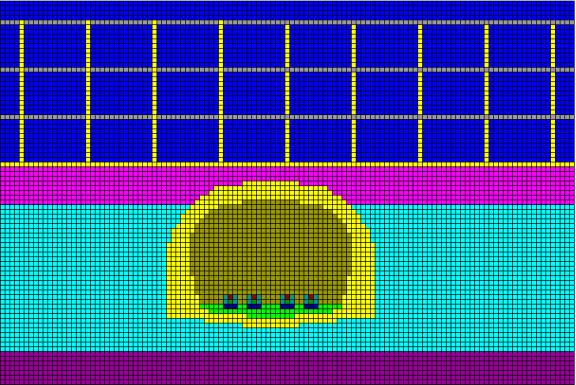
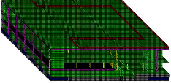
Figure 1 Cross section through model of brick tunnel with building above.
Figure 2
Isometric view of model of building for mixed use – Postal sorting office with residential units above
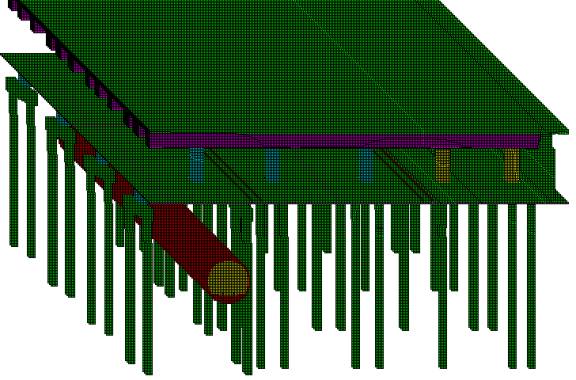
Figure 3
Isometric view of model of railway depot building on piled foundations above bored railway tunnel (soil around piles omitted for clarity)
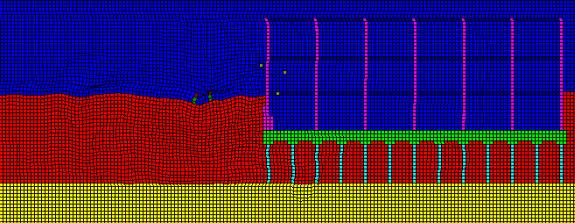
Figure 4
Instantaneous cross section through model of street-running tram adjacent to building founded on piles bearing on rock.
Output from the model is initially in the form of a time domain plot of, for the case of vibration, the displacement, velocity or acceleration, and in the case of airborne noise the sound pressure. Plots of this kind may be produced for all ro any cells in the model, the only cost being consumption of hard disk space and the large quantity of results.
The time domain plot may be converted to a .WAV file and replayed through loudspeakers if required for auralisation purposes. Otherwise it may be subjected to frequency transformation into either narrow band spectra or 1/3 octave frequency bands.
The vibration acceleration signal may be subjected to frequency weighting and the fourth-power integral obtained to give Vibration Dose Value. The airborne noise signal may be A-weighted and the square of the signal integrated in order to yield LAE (SEL) and thereby compute LAeq levels.
A typical example of the time-domain output is shown in figure 5, for the case of an impact due to the lowering of a mass on to the floor of the building shown in figure 25
Examples of narrow band and 1/3 octave band spectra are shown in figures 5 and 6.
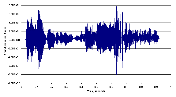
Figure 5
Time-domain output
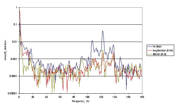
Figure 5
Example of narrow band output
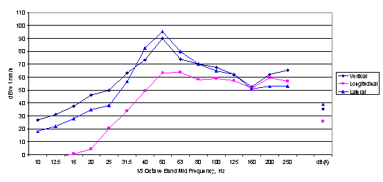
Figure 6
Example of 1/3 octave band output
Software Validation
The FINDWAVE® software package has been developed over the past ten years. That has been a long enough period for complex structures to have been modelled and constructed with opportunities to validate the predictions made using FINDWAVE®.
The following cases are instances where a FINDWAVE® model was created, in many cases during the design stage of the project, and field measurements were made to compare the predictions with actual results. There are of course two aspects to such a validation exercise, the first being the degree to which, for “true” assumptions about the cell properties in the model, the model correctly computes the response of the system. This is a test of the mathematical fidelity of the algorithm. The second aspect is the extent to which assumed assumptions and “true” assumptions coincide. For example, the dynamic properties of soils particularly loss factors are difficult to establish accuracy from soil investigations. Validation of assumptions is a separate matter from validation of the model itself, and should assumptions prove to have been incorrect, this is not a reflection on the validity of the model software, but rather on the coding of the properties of the cells in the model.
The first field validation work to be carried out was in 1994 when in a prediction exercise carried out in conjunction with the then CrossRail project to model airborne noise levels inside the Empire Theatre, Liverpool, England as a result of trains running in the Liverpool Loop tunnel. The model used was an early version of FINDWAVE® which used a polar grid rather than a rectangular grid, and did not include the ground surface or the actual theatre building. The tunnel was in sandstone, and the track directly fixed to a PACT (slip-formed concrete paved track) trackbed. The input data included measured rail roughness profiles from the actual tunnel. The prediction was done by modelling ground vibration at the position of the theatre building and than calculating the likely internal sound pressure sprectrum. This technique predicted the main peak in the spectrum at 80-Hz within some 2dB of the measured values.
In 1995 a FINDWAVE® model, also on the polar grid, was created of a main line railway tunnel in Germany, and prediction results compared with measurements of ground vibration due to the running of ICE trains. No data were available on wheel/rail roughness and a standard assumption was made. The results are shown in Figure 7.
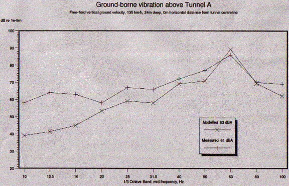
Figure 7 Comparison of measured and predicted levels of groundborne vibration from ICE trains in Germany.
Validation measurements were carried out in 1998 of FINDWAVE® predictions made in 1993 for the reconstruction of the District and Circle Line Station at Westminster, London. Here the new railway runs on a floating concrete slab on a suspended concrete bridge structure through the lower levels of the New Parliamentary building which was built above the deeply excavated new station for the Jubilee Line Extension.
Figure 8 shows a comparison of the measured vibration velocity in structural components of the New Parliamentary building with the FINDWAVE® predictions. Measurements of rail roughness had been made for the old District Line track before it was removed for the reconstruction of the station. It was assumed that the new track would be of the same (good) quality.
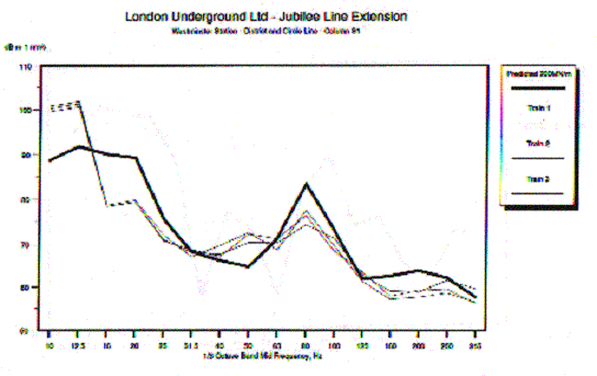
Figure 8
Comparison between measured vibration in column of New Parliamentary Building and FINDWAVE® predictions.
In 1999 A model verification exercise was carried out during the construction of the Copenhagen Metro in which the transmission loss between the tunnel floor and a room inside a building on the ground surface were measured and modelled. Results from this exercise are shown in figures 9 and 10.
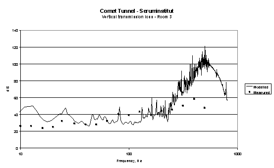
Figure 9
Comparison between measured and modelled transmission loss between base of Copenhagen Metro tunnel and room inside building above.
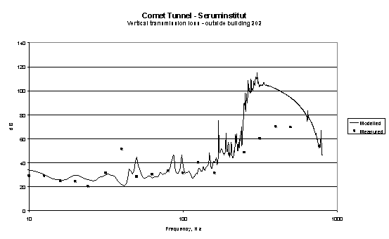
Figure 10
Comparison between measured and modelled transmission loss between bade of Copenhagen Metro tunnel and ground outside building above.
In 2001, measurements were made in a building located above the Jubilee Line Extension at a location close to the transition between floating track slab and resilient baseplate track. Measurements of a number of train passages were made and compared with predictions using FINDWAVE®. The results are compared in Figure 11. No rail or wheel roughness measurements were made, and a standard assumption for the roughness spectrum was assumed.
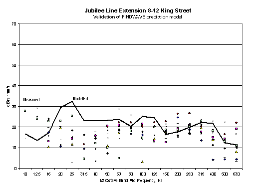
Figure 11
Model validation in basement of building above Jubilee Line Extension.
In 2002 a model was created of a bridge and adjacent structures carrying a tram system in Stockholm. The concrete deck abutting the bridge forms the roof of a “Teknikrum” and there are residential blocks immediately adjacent. The model was created to model airborne noise and structure-borne noise in and outside the adjacent buildings. For calibration purposes a tram vehicle was hauled by a locomotive over the bridge when it was partially complete, and comparisons made between the modelled and measured spectra, although the model was for a normal tram and the actual source was a locomotive hauled tram. The comparison in shown in figures 12 and 13.
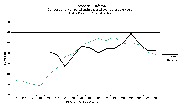
Figure 12
Comparison between measured noise from locomotive-hauled tram and computed noise from normal tram operation in room beneath tram bridge in Stockholm.
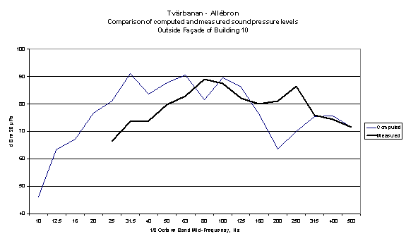
Figure 13
Comparison between measured noise from locomotive-hauled tram and computed noise from normal tram operation outside façade of building in Stockholm near to tram bridge.